Learned Relay Representations

Forward-thinking discrete diffusion via a learned latent channel trained with truncated BPTT.

This post is a companion walkthrough of our paper Learned Relay Representations for Forward-Thinking Discrete Diffusion Models. We summarize the motivation, the method, and the empirical findings in less technical prose; the full derivations, algorithm boxes, and ablations live in the paper.

Code: github.com/jacopo-minniti/relay

TL;DR. Standard masked diffusion throws away the rich hidden state computed at every denoising step and restarts from the discrete tokens alone. Relay keeps that state alive: at each step, the model’s last-layer hidden vector is projected and added back as a second input channel at the next step. Train the relay end-to-end with two-step truncated BPTT and it learns what to remember. On Sudoku-Extreme, this shifts the accuracy–NFE frontier outward; on a 1.5B-parameter coding LLM (Relay-finetuned Fast-dLLM v2), it beats vanilla SFT on HumanEval / MBPP with ~30% fewer forward passes.

Introduction

Masked Diffusion Models (MDMs) generate discrete sequences by iterative denoising: starting from a fully masked canvas $\mathbf{x}_{t_0}=(\textsf{[M]},\dots,\textsf{[M]})$, each forward pass unmasks a fraction of the remaining positions until the sequence is complete. Internally, the Transformer computes a rich hidden state at every position — including positions that are still masked — but at the end of each step those hidden states are thrown away. The next step starts again from the partially unmasked sequence alone.

We call this the hard reset problem. In standard MDMs, the only information that survives a denoising step is the discrete tokens just committed. The continuous, distributional reasoning the model just performed about every uncommitted position is wiped clean — and the next pass has to reconstruct it from scratch.

This matters because recurrent computation — unrolling a fixed-parameter model across many steps — is precisely the structural property recent work has tied to improved reasoning. MDMs already perform many forward passes per generation; the hard reset is what prevents any of that compute from compounding.

The question this post is about: How can the sequential unmasking structure of MDMs support recurrent computation that carries richer information across steps?

Our answer is Learned Relay Representations (Relay), a method that makes discrete diffusion models forward-thinking: at each denoising step, alongside any newly unmasked tokens, the model carries its last-layer hidden state forward as a learned relay. The next forward pass gets direct access to the prior step’s continuous computation. Simply piping these states forward, however, does not by itself ensure that they encode something useful for what follows. Relay therefore trains the relay end-to-end with truncated backpropagation through time (BPTT), shaping it to be maximally informative for the next few denoising steps.

Schematic of Relay over steps k and k+1: backbone f_theta, relay R_theta, hidden states h_k and h_{k+1}, progressive unmasking. — **Figure 1.** Schematic of Relay over two consecutive inference steps (as in the paper). At each step k, the backbone *f_θ* consumes the sum of embedded tokens *emb(x_{t_k})* and the projected relay state *R_θ(h_k)*, producing a hidden state h_k+1 that is both unembedded into logits for the cross-entropy loss and forwarded along the relay feedback path (highlighted in the paper figure) into the next step. Tokens are progressively unmasked between steps; h provides a continuous, differentiable channel for information that has not yet been committed to a discrete token.

Masked Diffusion Models in 60 Seconds

Before introducing the relay, it helps to be precise about what a standard MDM does and doesn’t carry across steps. We follow the formulations in.

Let $\mathcal{V}$ be a token vocabulary that includes a distinguished mask symbol $\textsf{[M]}$. Sequences live in $\mathcal{V}^L$. We write $\mathbf{x}_0 \in (\mathcal{V} \setminus {\textsf{[M]}})^L$ for a clean training sequence and $\mathbf{x}_t \in \mathcal{V}^L$ for its partially masked counterpart at noise level $t$.

Training

The noising process samples a time $t \in [0,1]$ and independently masks each position with probability $\alpha_t$, yielding $\mathbf{x}_t$. A neural network with backbone $f_\theta$, embedding $\textsf{emb}$, and unembedding $\textsf{unemb}$ parameterizes the per-position posterior

\[p_\theta^i(w \mid \mathbf{x}_t) = \frac{e^{\ell^i(w)}}{\sum_{w' \in \mathcal{V}} e^{\ell^i(w')}}, \qquad \ell^i(w) = \textsf{unemb}(f_\theta(\textsf{emb}(\mathbf{x}_t)))^i_w,\]

and is trained by minimizing the weighted cross-entropy

\[\mathcal{L}(\theta) = \mathbb{E}_{\mathbf{x}_0,\, t,\, \mathbf{x}_t} \!\left[ \frac{1}{t} \sum_{i:\, \mathbf{x}_t^i = \textsf{[M]}} -\log p_\theta^i\!\left(x_0^i \mid \mathbf{x}_t\right) \right].\]

Critically, only $\mathbf{x}_t$ is fed to the model: nothing about previous denoising steps is consumed.

Inference

Generation proceeds along a decreasing time grid $1 = t_0 > t_1 > \dots > t_K = 0$. At step $k$, the model computes logits $\boldsymbol{\ell}_k$ for the masked positions and an unmasking policy $u(\cdot \mid \boldsymbol{\ell}_k, \mathbf{x}_{t_k})$ commits a subset of positions, producing $\mathbf{x}_{t_{k+1}}$. Common choices include unmasking a fixed fraction per step or confidence-based parallel decoding.

The Hard Reset Problem

After each inference step, MDMs discard the entire computational state used to choose the newly revealed tokens. Step $k{+}1$ starts again from $\mathbf{x}_{t_{k+1}}$ alone. Standard MDM inference therefore treats every partially masked sequence as a fresh prediction problem rather than as a continuation of an ongoing computation. Because models can only perform a constant number of FLOPs per forward pass, this hard reset prevents the model from amortizing reasoning across steps. Related observations have been made under the names information island and sampling wall.

Augmented State Trajectories

Our fix is to introduce a continuous, differentiable channel alongside the discrete one. We augment the inference state from $\mathbf{x}_{t_k}$ to the pair

\[\mathbf{s}_{t_k} \;=\; \bigl(\mathbf{x}_{t_k},\, \mathbf{h}_{t_k}\bigr),\]

where $\mathbf{h}_{t_k}$ is the last-layer hidden state produced at step $k$. We can decompose the desired behavior into two primitives the model must learn:

Produce a useful relay $\mathbf{h}_{t_k}$ at step $k$.
Consume $\mathbf{h}_{t_k}$ at step $k{+}1$.

Concretely (cf. Figure 1), at each step the backbone reads the sum of token embeddings and a projected relay,

\[\mathbf{h}_{k+1} \;=\; f_\theta\!\bigl(\,\textsf{emb}(\mathbf{x}_{t_k}) + R_\theta(\mathbf{h}_{t_k})\,\bigr), \qquad \boldsymbol{\ell}_k \;=\; \textsf{unemb}(\mathbf{h}_{k+1}),\]

where $R_\theta$ is a small relay module that lives in the same residual stream as the token embeddings.

Two things are worth emphasizing:

The relay $\mathbf{h}_{t_k}$ is an internal model state, not an externally observed conditioning variable. At inference, each step forwards the pair $(\mathbf{x}_{t_k}, \mathbf{h}_{t_k})$, but only $\mathbf{x}_{t_k}$ is ever decoded into text.
Relay leaves the inference-time decoding procedure (unmasking schedule, sampling rule) unchanged. The only addition at inference is shipping the relay alongside the committed tokens.

Training the Relay with Truncated BPTT

A relay channel that is passed forward but never trained to be useful will not learn to carry the right information. So during training we unroll the augmented state for $K$ steps, accumulate the standard cross-entropy loss across the rollout, and backpropagate through the relay path via truncated BPTT:

\[\mathcal{L}_K(\theta;\, \mathbf{x}_0,\, \xi_{0:K-1}) \;=\; \sum_{k=0}^{K-1} L_k(\boldsymbol{\ell}_k,\, \mathbf{x}_0).\]

Each per-step loss $L_k$ is the cross-entropy on the masked positions of the corresponding rollout state. Importantly, we treat the discrete update $\mathbf{x}_{t_k} \mapsto \mathbf{x}_{t_{k+1}}$ as fixed after sampling — that is, we do not differentiate through the sampled unmasking decisions. Gradients flow into $\theta$ both directly through the logits at each step and temporally through the differentiable relay path $\mathbf{h}_k \to \mathbf{h}_{k+1}$.

Training procedure

Algorithm 1 in the paper instantiates one outer optimization step: maintain a rollout buffer state $(z, \mathbf{h})$, run $K$ inner relay steps with teacher-forced unmasking under policy $u$, accumulate cross-entropy, and apply a gradient step. The figure below matches the manuscript.

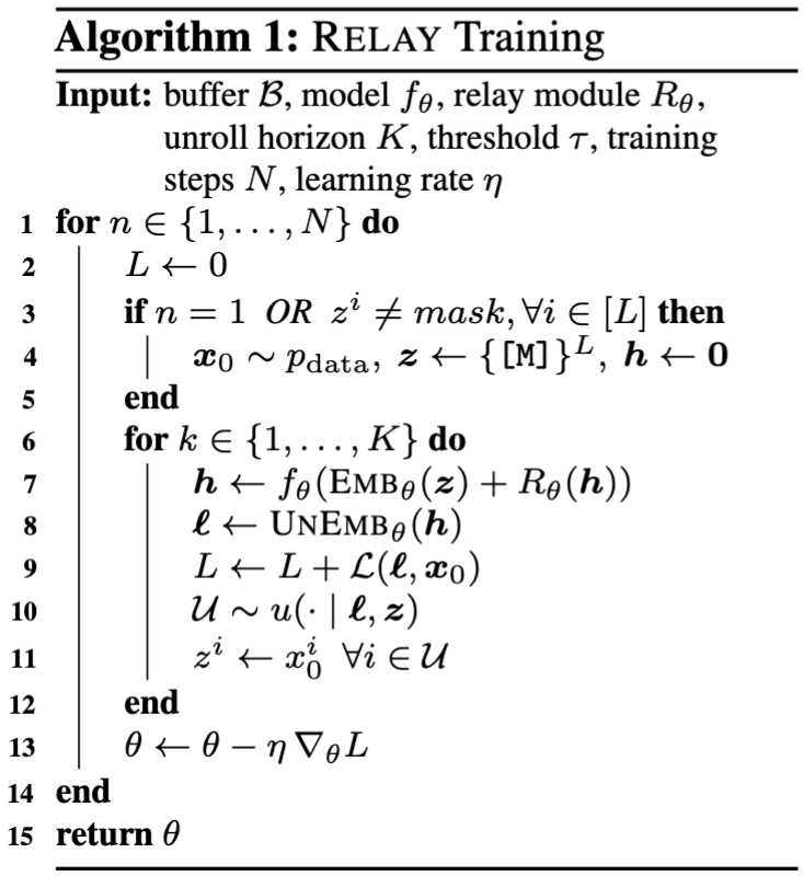
Algorithm 1: Relay training — outer loop over training steps, inner K-step rollout with embedding, relay R_theta, forward f_theta, unembed, loss, unmasking, gradient update. — **Figure 2.** **Algorithm 1:** Relay training (one outer iteration). Inner loop: update hidden state via *f_θ* on embedded tokens plus *R_θ(h)*, compute logits and loss, sample unmasking positions, teacher-force commits from x₀, then apply *θ ← θ − η ∇_θL*.

Constructing rollouts

Given the current augmented state $(\mathbf{x}_{t_k}, \mathbf{h}_{t_k})$, one rollout step proceeds as:

Unmasking. Sample positions $\mathcal{U} \sim u(\cdot \mid \boldsymbol{\ell}_k, \mathbf{x}_{t_k})$ using the same on-policy confidence sampler we use at inference.
Token selection. Teacher-force the unmasked positions to the ground-truth values: $x_{t_{k+1}}^i = x_0^i$ for $i \in \mathcal{U}$. Without teacher-forcing the model is exposed to its own early mistakes, which it has no mechanism to correct during the rollout.

This rollout scheme leaves the ideal minimizer unchanged from the standard MDM objective; intuitively, sampling positions on-policy and teacher-forcing their values does not alter what the right answer is, only the distribution over which contexts the model practices on.

Two-step gradients

In our experiments we use the minimal non-trivial truncation horizon, $K{=}2$: the model rolls out two consecutive steps, and the second step’s cross-entropy gradient flows back through the relay into the first step’s hidden state. This is enough to give the model an explicit incentive to encode information at step $k$ that pays off at step $k{+}1$, without paying a long-horizon BPTT bill.

Concretely, the two-step gradient decomposes into the usual local term plus a BPTT correction routed through the relay path; we give the full adjoint recursion in §3.2 of the paper.

Validating the Design on Sudoku

We first study Relay on Sudoku-Extreme, a 9×9 logical-reasoning puzzle with a unique solution. Sudoku is a clean test bed: it has a small vocabulary, an obvious notion of legality at every partial state (no row/column/box repeats), and rich global constraints that should reward a model that can carry intermediate reasoning across steps.

Setup

All methods use the same small Transformer backbone (~7M parameters) with rotary position embeddings, trained to convergence. To isolate the contribution of each ingredient of Algorithm 1 (Figure 2) in the paper, we compare four objectives, each in tied- and untied-embedding variants:

MLM — standard uniform masked diffusion ($K{=}1$, no relay).
Rollout — $K{=}2$ on-policy rollouts, but no relay ($R_\theta \equiv 0$).
Relay (sg) — $K{=}2$ relay rollouts, but stop-gradient on the relay between steps (no temporal credit).
Relay — the full method: $K{=}2$ BPTT through the relay.

At inference, we sweep deterministic confidence thresholds $\tau \in {0.05, 0.10, 0.15, 0.20, 0.25}$ and trace each method’s accuracy–NFE frontier. Lower $\tau$ commits fewer cells per forward pass and so spends more NFEs.

The accuracy–NFE frontier

Sudoku token accuracy versus average rollout steps (NFE). — **Figure 3.** Accuracy–NFE frontiers on Sudoku-Extreme. Each curve traces a single training method as we sweep the inference confidence threshold; shaded ribbons are ±1 sample std. across three training seeds.

Sudoku exact-match accuracy versus average rollout steps (NFE). — **Figure 3.** Accuracy–NFE frontiers on Sudoku-Extreme. Each curve traces a single training method as we sweep the inference confidence threshold; shaded ribbons are ±1 sample std. across three training seeds.

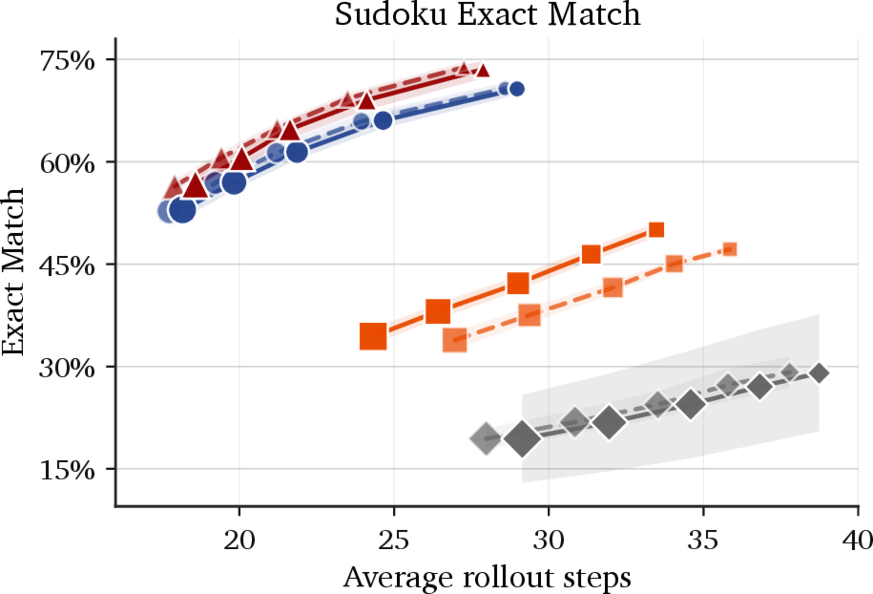
Reading the transitions in Figure 3 from baseline to best-performing:

MLM → Rollout. Replacing uniform masking with an on-policy confidence-thresholded sampler under teacher forcing already moves the frontier substantially. The lesson: aligning what is masked during training with what gets revealed at inference matters even before introducing any relay.
Rollout → Relay (sg). Adding the relay channel — even with a stop-gradient between steps — yields the next big jump. A continuous handoff between forward passes provides value even when it is not yet trained for that handoff.
Relay (sg) → Relay. Replacing the stop-gradient with $K{=}2$ BPTT through the relay gives a further separation and the best frontier across thresholds. Training the relay to be useful, not just letting one exist, is the dominant effect.

Why BPTT helps the relay

What does the relay learn under BPTT? We trace the separation between Relay and Relay (sg) to a concrete behavior: at the same threshold $\tau$, Relay commits more cells per forward pass while keeping the partial board legal. A board is legal when no row, column, or 3×3 box contains a repeated digit; legality is necessary (but not sufficient) for correctness, and is defined at every intermediate denoising step, not only at the end.

At the matched threshold $\tau = 0.15$ on a deduction-only subset of 2,000 puzzles, Relay produces a fully legal final board 74.8% of the time versus 70.7% for Relay (sg) (+4.1 pp), and incurs 15% fewer row/column/box violations across the rollout (0.90 vs. 1.06 per puzzle). The improvement holds uniformly across both Advanced and Master difficulty strata.

In other words, BPTT teaches the relay to keep the partial board self-consistent under more aggressive unmasking: at the same confidence threshold, Relay commits more cells per pass while still honoring the global constraints, so the rollout reaches the same accuracy in fewer total forward passes — exactly the outward shift of the frontier in Figure 3.

Scaling to Fast-dLLM v2

Sudoku tells us what Relay buys when trained from scratch. To see whether the same recipe holds at LLM scale, we adapt a pretrained DLM — Fast-dLLM v2 (1.5B) — into a Relay model with a small amount of supervised finetuning.

Block diffusion and KV caching

Fast-dLLM v2 combines block-autoregressive decoding in the style of Block Diffusion with KV caching for previously decoded blocks. To make our two-step relay rollout compatible with this:

Per-block rollout. The $K{=}2$ rollout runs only inside the active block, leaving previously decoded blocks frozen so their inter-block KV cache is reused unchanged across both passes.
Mask-only relay updates. Within the active block we update the relay state only at positions that are still masked. Already-committed sub-block tokens still contribute attention, but their relay entries are not overwritten — keeping within-block sub-block KV cache entries valid as the block fills in.

With these two adaptations, Algorithm 1 plugs in cleanly without breaking Fast-dLLM v2’s acceleration story.

Coding results

We finetune all parameters for 200 optimizer steps at effective batch size 32 on a 60k-example 40/60 code/math mixture of OpenCodeInstruct and OpenMathInstruct-2 (details in the paper). Inference follows Fast-dLLM v2’s confidence-based parallel decoding at $\tau=0.85$.

Method	HumanEval (Base)	HumanEval (Plus)	HumanEval NFE	MBPP (Base)	MBPP (Plus)	MBPP NFE
Fast-dLLM v2 (1.5B)	38.4%	35.4%	178.1	46.8%	39.7%	133.0
Vanilla SFT	38.4%	34.1%	130.7	43.9%	38.1%	84.8
Relay (sg)	38.4%	35.4%	104.4	43.1%	39.2%	80.1
Relay	42.1%	37.2%	88.3	46.6%	41.5%	78.8

The same pattern from Sudoku reappears at LLM scale: Relay attains the best accuracies and the lowest NFE among adapted methods on both HumanEval and EvalPlus variants. Notably, on HumanEval, Relay surpasses Vanilla-SFT’s accuracy while spending 32% fewer NFEs (88.3 vs. 130.7) — the relay-trained model is simultaneously more accurate and faster than its non-relay counterpart finetuned on identical data.

Training Memory

A reasonable worry is that BPTT through $K{=}2$ forward passes doubles training memory. We profiled one micro-step on an A100 80GB, and it does not — and the reason turns out to be structural, rooted in how Fast-dLLM v2’s vanilla SFT forward is shaped versus how Relay’s rollout forwards are shaped.

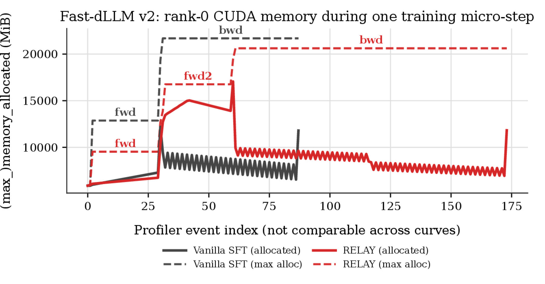
GPU memory: vanilla SFT vs. Relay during one micro-step. — **Figure 4.** GPU memory during one training micro-step of Fast-dLLM v2 on an A100 80GB. Solid lines show live GPU memory at every decoder-layer fwd/bwd hook; dashed lines show the running high-water mark within the micro-step. Note that Relay's first forward (red `fwd1`) plateaus at roughly *half* the forward-pass footprint of vanilla SFT's single forward (black `fwd1`) — the direct consequence of the input-shape asymmetry below.

The shape asymmetry. Both regimes inherit BD3-LM’s $[\mathbf{x}_t \,|\, \mathbf{x}_0]$ layout, which concatenates the noised and clean sequences and so doubles the sequence dimension to $2L$. Vanilla SFT, however, additionally makes a complementary-mask copy along the batch dimension, doubling it to $2B$. So a single vanilla forward runs at shape $(2B, 2L)$, whereas each of Relay’s two rollout forwards runs at the undoubled batch, $(B, 2L)$. That is exactly why, in Figure 4, Relay’s red fwd1 adds about half the activation memory of vanilla’s black fwd1: same $2L$, half the batch. Two Relay forwards at $(B, 2L)$ together demand memory comparable to vanilla’s one forward at $(2B, 2L)$.

Two asymmetries that roughly cancel. The binding peak of the micro-step in both regimes is the cross-entropy backward through the vocab projection head (lm_head), which materializes a $B \times T \times V$ fp32 grad-of-logits buffer. Because vanilla carries the doubled batch into that backward, its buffer is twice as large as Relay’s: at per-device batch size 2 with $T=2048$, $V=151{,}936$, it is $[4, 2048, 151936]\times 4\,\text{B} \approx 4.6$ GiB for vanilla versus only $\approx 2.3$ GiB for Relay. Relay spends its savings on the activation side instead: its second forward raises live memory by roughly 5 GiB through fwd2 (forward 1’s saved activations and the relay state $\mathbf{h}$ must coexist with forward 2 to route credit through both passes), though most of that is autograd intermediates rather than saved-for-backward state, and PyTorch releases it in a single step before the lm_head spike fires.

The result: peak memory is 20.1 GiB for Relay vs. 21.2 GiB for vanilla SFT — within ~1 GiB. The near-tie is structural, not allocator-timing noise: Relay simply trades vanilla’s in-forward batch doubling for an explicit second pass. BPTT through $K{=}2$ therefore does not double peak memory in this setup (gradient checkpointing, ZeRO-3, non-fused CE), and we expect peak memory to stay comparable whenever the vanilla baseline already pays a doubled-batch forward and the lm_head backward dominates.

Takeaways

The hard-reset bottleneck in masked diffusion has a clean fix: give the model a differentiable channel between steps, and train it to be useful with truncated BPTT.

Stepping back:

A continuous relay channel is the structural minimum needed to break the hard reset. Even with a stop-gradient it already improves the Pareto frontier.
BPTT through the relay is what makes the relay learn what to remember. On Sudoku, this shows up as more aggressive but still legal unmasking; on Fast-dLLM v2, as simultaneously higher accuracy and fewer NFEs.
The recipe is architecture-agnostic, leaves the inference decoding procedure unchanged, and is compatible with prevalent DLM acceleration techniques like block diffusion and KV caching — so it composes with the same engineering stack used in state-of-the-art diffusion LLMs.

If you found this useful, please consider citing our paper:

@inproceedings{rozonoyer2026relay,
  title     = {Learned Relay Representations for Forward-Thinking Discrete Diffusion Models},
  author    = {Rozonoyer, Benjamin and Minniti, Jacopo and Patel, Dhruvesh and Band, Neil and Bose, Joey and Rudner, Tim G. J. and McCallum, Andrew},
  booktitle = {Structured Probabilistic Inference \& Generative Modeling (SPIGM) and Frontiers in Generative AI (FoGen) Workshops at ICML},
  year      = {2026}
}